Moving Beyond Arbitrary Percentiles: Data-Driven Biomarker Cutoffs with Gaussian Mixture Models

In biomarker research, one of the most consequential decisions is also one of the least discussed: how do you define “high” versus “low” expression?

The most common approach is to pick a percentile — median split, upper tertile, upper quartile — and use it as the cutoff. Percentile-based cutoffs are widely used because they’re simple, reproducible, and easy to standardize across studies. The problem is that they’re often biologically arbitrary. The biology doesn’t care about your 67th percentile.

There’s a better way.

The Problem with Percentile-Based Cutoffs

Percentile cutoffs assume that the population is uniformly distributed along the expression axis and that a fixed fraction of samples should fall into the “high” category. Neither assumption is usually true.

Consider a biomarker where 80% of tumors genuinely express it at high levels and 20% do not. A median split would classify half the high-expressors as “low,” diluting your treatment group and reducing statistical power. Conversely, if only 15% of tumors are truly high-expressors, a tertile cutoff would contaminate your “high” group with samples that don’t actually overexpress the target.

The result: clinical trials with inflated enrollment, muddy response signals, and companion diagnostics that don’t perform as expected.

Gaussian Mixture Models: Finding Natural Populations

Gaussian Mixture Models (GMMs) offer a data-driven alternative (Fraley & Raftery, 2002). Instead of imposing an arbitrary dividing line, GMMs ask: does the expression data naturally separate into distinct populations?

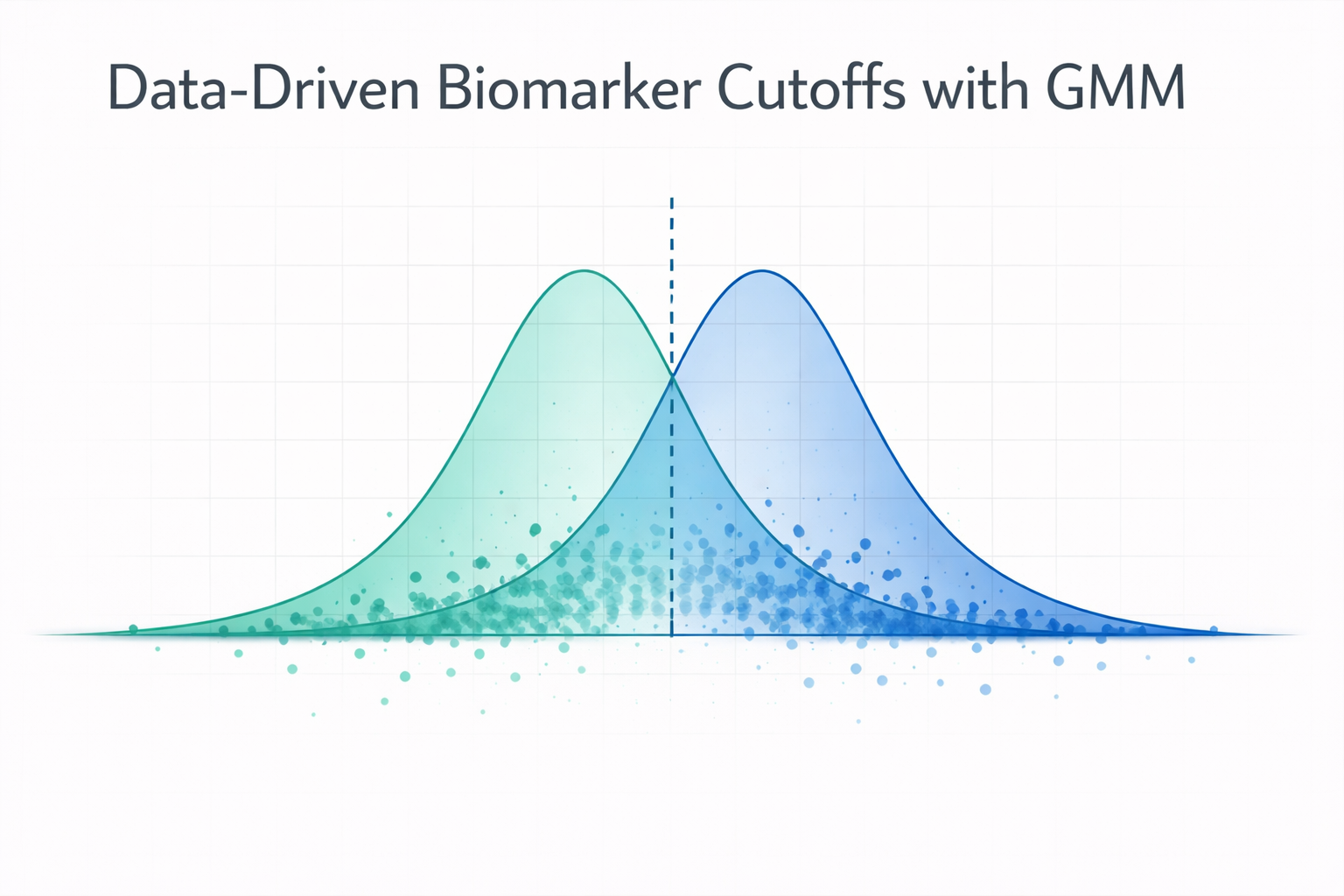
Conceptually, GMM asks whether your data is best explained as a single population or a mixture of distinct biological groups. It fits the observed expression distribution as a weighted sum of Gaussian (normal) distributions. For a two-component GMM:

• Component 1 captures the “low expression” population with its own mean and variance
• Component 2 captures the “high expression” population with its own mean and variance
• The intersection point between the two Gaussians becomes the natural cutoff

This approach has several advantages:

1. Biologically motivated: If a biomarker truly defines two patient populations, the GMM will find them — an approach that has been applied successfully in cancer classification (Prabakaran et al., 2019). If the distribution is unimodal, the GMM will tell you that too — which is equally valuable information.
2. Adaptive: The cutoff adjusts to your specific dataset rather than being fixed at an arbitrary fraction.
3. Quantified uncertainty: GMMs provide posterior probabilities for each sample’s group membership, so you know which samples are confidently classified versus borderline.

A Practical Example

Imagine you’re studying expression of a therapeutic target across 300 tumor samples. The expression values (log2-transformed, normalized) range from 8 to 15.

• Tertile cutoff (67th percentile): Cutoff at 11.07, classifying 33% as “High”
• GMM cutoff: Identifies two natural populations centered at 10.2 and 13.1, with an optimal separation at 11.70, classifying 61% as “High”

The GMM reveals that the majority of tumors actually express this target at high levels — a finding with direct implications for clinical trial design and patient eligibility. In this scenario, the biology suggests the target is broadly expressed rather than confined to a small subset. The tertile approach would have excluded a large fraction of eligible patients.

When to Use Each Approach

GMMs are not always superior. Here’s a decision framework:

Scenario	Recommended Approach
Biomarker with known bimodal distribution	GMM
Exploratory analysis, unknown distribution	GMM (to characterize the data), then validate
Small sample size (n < 30)	Percentile (GMM needs sufficient data to fit reliably)
Regulatory submission requiring predefined cutoff	Percentile (for reproducibility), but validate with GMM
Comparing across datasets	Percentile (unless GMMs are fit per-dataset)

Implementation Tips

Once you’ve confirmed that a bimodal structure is plausible, fitting a GMM is straightforward:

In R

# Fraley & Raftery, 2002
library(mclust)
fit <- Mclust(expression_values, G = 2)
cutoff <- optimize(function(x) {
  abs(dnorm(x, fit$parameters$mean[1], sqrt(fit$parameters$variance$sigmasq[1])) *
      fit$parameters$pro[1] -
      dnorm(x, fit$parameters$mean[2], sqrt(fit$parameters$variance$sigmasq[2])) *
      fit$parameters$pro[2])
}, interval = range(expression_values))$minimum

In Python

# Pedregosa et al., 2011
from sklearn.mixture import GaussianMixture
import numpy as np

gmm = GaussianMixture(n_components=2, random_state=42)
gmm.fit(expression_values.reshape(-1, 1))

# Find intersection
x_range = np.linspace(expression_values.min(), expression_values.max(), 1000)
probs = gmm.predict_proba(x_range.reshape(-1, 1))
cutoff = x_range[np.argmin(np.abs(probs[:, 0] - probs[:, 1]))]

Validation Checklist

• Never rely on GMM alone — confirm bimodality visually (histogram + density plot)
• Cross-validate with K-means and KDE (kernel density estimation)
• Evaluate model fit using BIC — if a one-component model fits nearly as well, the data may not be truly bimodal
• Check that the GMM cutoff produces biologically coherent groups
• If tissue-type specific, apply the cutoff only to the relevant compartment

A Note of Caution

GMMs can overfit if the data is not truly multimodal. A two-component model will always find two components — even when the underlying distribution is unimodal — by splitting a single population in half. Always evaluate model selection criteria such as BIC (Schwarz, 1978) and confirm structure visually before interpreting the results. If the BIC difference between one-component and two-component models is marginal, the data may not support a bimodal cutoff.

The Compartment Question

One subtlety we’ve encountered in spatial biology: the compartment in which you define the cutoff matters enormously. An epithelial biomarker should be stratified using expression measured in the epithelial/tumor compartment — not from pooled data that includes stroma and immune regions where the marker has different expression dynamics.

Using the wrong compartment can shift your cutoff by a full log2 unit or more, fundamentally changing which samples are classified as “high” and altering downstream conclusions.

Bottom Line

Biomarker cutoff selection is not a statistical formality. It directly affects patient stratification, clinical trial design, and therapeutic decision-making. Data-driven methods like GMMs provide a principled alternative to arbitrary percentiles — one that respects the underlying biology and adapts to the data.

These decisions aren’t just statistical — they directly impact how patients are stratified and how therapies are evaluated. At Cytogence, we routinely apply GMM-based stratification in our spatial transcriptomics and biomarker analysis workflows. If you’re developing a companion diagnostic or stratifying patients for a clinical study, a data-driven cutoff isn’t just better statistics — it’s better science.

References

1. Fraley C, Raftery AE. Model-based clustering, discriminant analysis, and density estimation. Journal of the American Statistical Association. 2002;97(458):611-631. doi: 10.1198/016214502760047131.

2. Schwarz G. Estimating the dimension of a model. The Annals of Statistics. 1978;6(2):461-464.

3. Prabakaran I, Wu Z, Lee C, et al. Gaussian mixture models for probabilistic classification of breast cancer. Cancer Research. 2019;79(13):3492-3502. doi: 10.1158/0008-5472.CAN-19-0573. PMID: 31113820.

4. Pedregosa F, Varoquaux G, Gramfort A, et al. Scikit-learn: machine learning in Python. Journal of Machine Learning Research. 2011;12:2825-2830.

---

Cytogence helps research teams turn complex biological data into clear, defensible results. Learn more about our bioinformatics services.