Batch Effects in RNA-seq: How to Catch Them Before They Wreck Your DE Results

The first PCA plot tells you everything. On a recent bulk RNA-seq project, the samples didn’t separate by treatment — they separated, cleanly and depressingly, by the week they were sequenced. Two libraries had been prepped a month after the rest, on a new kit lot, and that single operational detail was now the loudest signal in the dataset. The biology was in there somewhere, underneath a technical gradient that no amount of downstream cleverness was going to wish away.

This is the batch-effect problem, and it is not exotic. Anytime samples are processed in groups — different days, kit lots, operators, flow cells, extraction protocols, or sites — you risk a systematic, non-biological difference between those groups that masquerades as signal. The danger isn’t that batch effects exist; it’s that they’re invisible in a gene list. A volcano plot from a batch-confounded analysis looks exactly as convincing as a real one. So the discipline is to catch the problem upstream, decide honestly whether it’s fixable, and then choose the lightest intervention that actually works. Here’s how we approach it.

Detect before you correct

The instinct to immediately “remove the batch effect” is the wrong first move. You first need to know whether you have one, how strong it is, and — critically — whether it’s tangled up with the thing you care about. A handful of diagnostics do most of the work:

PCA, colored by every metadata variable you have. Plot variance-stabilized counts (VST, or rlog for very small datasets) and color the points by treatment, by batch, by sequencing date, by RIN, by library prep day — one plot per variable. Color by technical QC metrics too: sequencing depth, mapping rate, and duplication rate often explain structure that no biological label accounts for. If PC1 or PC2 lines up with a technical variable instead of your biology, you’ve found your problem — though important batch structure can also surface in later principal components when strong biological variation dominates the first few, so don’t stop at PC1/PC2. This is often the most informative diagnostic in the analysis.
Hierarchical clustering / sample correlation heatmap. Cluster samples and annotate the dendrogram with batch and condition. Samples should generally cluster according to known biological structure rather than technical processing variables. If they group by batch, the batch effect dominates.
Quantify it on larger studies. When you have the sample size for it, variance-partitioning approaches (variancePartition) can estimate how much of each gene’s expression variability is attributable to batch versus treatment, donor, site, or other covariates — turning the qualitative PCA impression into a number you can defend.
The metadata you should already have. None of this works if you don’t know the batches. Sequencing date, kit lot, prep operator, and site belong in your sample sheet from day one. The most common reason a batch effect goes uncorrected isn’t a hard analysis — it’s that nobody recorded which samples were processed together. Capture it before it’s lost.

The 2024 Genome Biology review by Yu and colleagues makes the same point at consortium scale: detection and disciplined experimental design come first, and visualization (PCA and related projections) remains the front-line tool for spotting the problem (Yu et al., 2024).

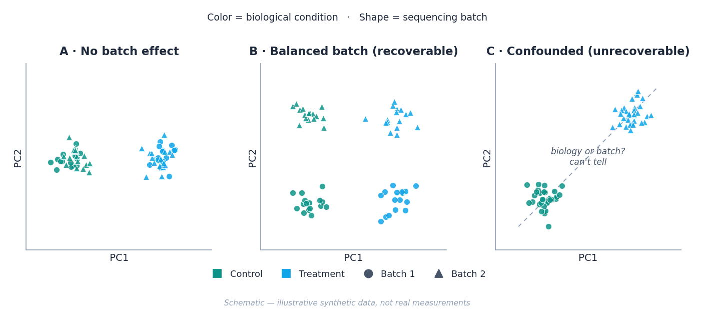Schematic: the danger isn’t batch effects — it’s batch effects that overlap with biology. A batch you can model out (B) is a nuisance; a batch confounded with condition (C) is a dead end.

The trap you can’t fix: confounding

Before you touch a correction method, ask the question that determines whether any of them will help: is batch confounded with my condition of interest?

If all your treated samples were sequenced in batch 1 and all your controls in batch 2, then “treatment” and “batch” are the same variable wearing two names. No statistical method — not ComBat-seq, not SVA, not putting batch in the model — can separate an effect from a covariate it perfectly tracks. The math simply has no information to work with. We’ve had to deliver this news on real projects, and it never lands gently: the honest answer is that the experiment, not the analysis, needs to change.

This is why the cheapest batch-effect insurance is bought at the bench, not the keyboard. Randomize and balance your samples across batches so that each batch contains a mix of conditions. Partial balance is recoverable; total confounding is not. If you’re designing the study now, this is the single highest-leverage paragraph in this post.

Confounding also isn’t all-or-nothing — most real datasets aren’t perfectly confounded, just ugly. Imagine a design where batch 1 holds eight controls and one treated sample while batch 2 holds the reverse: the model can in principle separate batch from treatment, but it has very little information to do so. Power drops and the estimates get unstable. The closer batch and condition drift toward each other, the less the model has to separate them — long before they collapse into perfect confounding.

The default move: model batch, don’t erase it

When batch is known and not fully confounded, the best practice is also the simplest one — and it’s not “correct the counts.” It’s to add batch to your design formula and let the differential-expression model account for it:

# DESeq2: control for batch while testing treatment
design(dds) <- ~ batch + treatment

edgeR and limma do the same thing with batch as a covariate in the linear model. The variable you test for differential expression goes last; everything before it is “adjusted for.” This keeps the analysis on raw counts — which is where DESeq2 and edgeR’s dispersion estimation and statistics are designed to operate — and it propagates the uncertainty correctly into your p-values. Current Bioconductor guidance and many comparative studies favor this: when the differential-expression framework supports covariates, modeling a known batch beats generating a separately “corrected” count matrix and pretending the correction was free (Yu et al., 2024; Zhang et al., 2020).

There’s an important corollary about the batch-corrected plots you do want to make. To produce a PCA that visually removes batch, limma::removeBatchEffect() is the right tool — but its own documentation is blunt about the boundary: it is for plotting and exploration only, not for linear modeling and differential expression (Ritchie et al. / limma docs). Feeding batch-corrected values back into a DE test double-counts the correction and inflates significance. Correct the counts to see the biology; model the batch to test it. Those are two different operations, and conflating them is one of the most common ways a batch-aware analysis quietly goes wrong.

When you genuinely need corrected counts: ComBat-seq

Sometimes you can’t model batch in the design — most often when you’re integrating datasets for a downstream tool that takes a single expression matrix and offers no covariate slot (some clustering, visualization, or machine-learning workflows), or when you’re pooling studies for a meta-analysis. For RNA-seq counts, ComBat-seq (in the sva package) is the workhorse: it adapts the original microarray ComBat to count data using a negative binomial regression, so the output remains integer-valued and can be used in downstream count-based workflows — though when batch is known and can be modeled directly, the DESeq2 and edgeR developers generally recommend including batch in the design rather than batch-correcting the counts first (Zhang et al., 2020).

Two honest caveats. First, ComBat-seq needs batch labels — it corrects known batches, not mystery variance. Second, even well-applied count correction generally yields lower statistical power than data that never had a batch effect, and over-aggressive correction can erase real biology along with the noise. Reach for count correction when the workflow forces your hand, not as a reflex.

When the batch is hidden: SVA and RUVSeq

The hardest case is the batch effect you can’t name — unmeasured technical variation with no label to model. Two families of methods estimate that hidden structure directly from the data:

SVA / svaseq estimates surrogate variables — latent factors capturing unwanted variation — that you then add to your design formula alongside your known covariates (Leek et al., svaseq).
RUVSeq removes unwanted variation using negative-control genes (housekeeping genes or spike-ins assumed not to respond to your treatment) or technical replicates to anchor the estimate (Risso et al., 2014). It is only as good as those controls: control genes that quietly respond to the biology of interest will bias the correction.

Both let you account for hidden batch inside the model, which keeps them in the philosophically preferable “adjust, don’t erase” camp. The catch is that they’re easier to misuse: surrogate variables can absorb genuine biological signal if your design or control genes are poorly chosen, silently deflating the effect you came to find. These are powerful tools that reward knowing exactly what they assume — and punish running them on defaults.

What this looks like in practice

There’s no universal recipe, but the order of operations is stable. Detect first — PCA and clustering against full metadata. Check for confounding, and say so plainly if the design can’t support the question. If batch is known and the design allows it, model it (~ batch + treatment) and stay on raw counts. If a downstream tool forces a single corrected matrix, use ComBat-seq and accept the power cost. If the batch is unmeasured, reach carefully for SVA or RUVSeq with controls you can defend. And whatever you do to the counts for a plot, never let those plotted values masquerade as test input.

The thread running through all of it: batch effects are a data-quality problem first, a statistics problem second. The analyses that go wrong usually didn’t pick the wrong correction method — they skipped the detection step, or inherited a confounded design nobody flagged, or quietly fed corrected values into a significance test. Catch it on the first PCA plot and most of the downstream pain never happens.

Batch effects are where a lot of RNA-seq projects silently lose their conclusions, and diagnosing one in someone else’s pipeline is a routine part of our work. If you’re staring at a PCA that’s clustering by sequencing date instead of biology — or you want a design reviewed before you spend the sequencing budget — our RNA-seq analysis service handles exactly this.

References

Yu Y, Mai Y, Zheng Y, Shi L. Assessing and mitigating batch effects in large-scale omics studies. Genome Biology. 2024;25:254. doi: 10.1186/s13059-024-03401-9.
Zhang Y, Parmigiani G, Johnson WE. ComBat-seq: batch effect adjustment for RNA-seq count data. NAR Genomics and Bioinformatics. 2020;2(3):lqaa078. doi: 10.1093/nargab/lqaa078.
Leek JT. svaseq: removing batch effects and other unwanted noise from sequencing data. Nucleic Acids Research. 2014;42(21):e161. doi: 10.1093/nar/gku864.
Risso D, Ngai J, Speed TP, Dudoit S. Normalization of RNA-seq data using factor analysis of control genes or samples (RUVSeq). Nature Biotechnology. 2014;32(9):896-902. doi: 10.1038/nbt.2931.
Ritchie ME, Phipson B, Wu D, et al. limma powers differential expression analyses for RNA-sequencing and microarray studies. Nucleic Acids Research. 2015;43(7):e47. removeBatchEffect documentation. doi: 10.1093/nar/gkv007.

Cytogence is the bioinformatics division of KeyQ, Inc. We help research teams design RNA-seq experiments and analyze them rigorously. See how we approach RNA-seq.