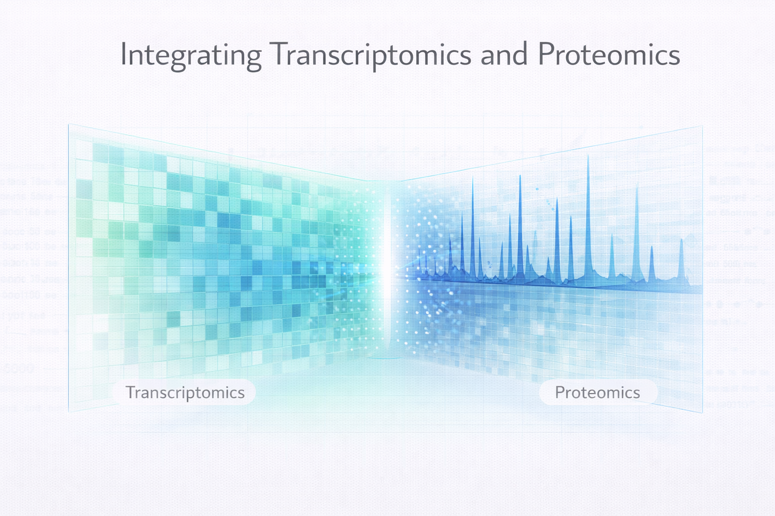
Integrating Transcriptomics and Proteomics: A Practical Guide

RNA tells you what the cell plans to make. Protein tells you what it actually made. The gap between plan and execution is where some of the most interesting biology lives — and in most datasets, that gap is larger than people expect.

Integrating transcriptomics (RNA-seq) and proteomics (LC-MS/MS or spatial protein profiling) is increasingly common in modern research. But the integration is rarely as simple as “merge the tables and correlate.” The challenge is that these modalities measure fundamentally different layers of biology, with different noise profiles and detection biases. Here’s what we’ve learned from doing it in practice.

Why Integrate?

Each technology captures a different slice of cellular activity:

Feature	Transcriptomics	Proteomics
Coverage	15,000-20,000 genes	2,000-10,000 proteins (LC-MS) or hundreds (targeted panels)
Dynamic range	Very high (6+ orders of magnitude)	Moderate (3-4 orders of magnitude)
Sensitivity to low-abundance molecules	Good	Poor (biased toward high-abundance proteins)
Reflects post-translational modifications	No	Yes (with appropriate methods)
Turnaround time	Hours (sequencing) to days	Hours to days (mass spec)
Biological meaning	Transcriptional state	Functional state

These differences explain why direct one-to-one comparisons often fall short. But integration still adds value in three important ways:

1. Validation: Findings supported by both RNA and protein are more robust than single-modality results
2. Discovery: Discordant genes — where RNA and protein disagree — point to post-transcriptional regulation, protein stability mechanisms, or translational control
3. Completeness: Pathways that are only partially visible in one modality may become fully resolved when both are combined

The ID Mapping Problem

Before you can compare RNA and protein, you need to map between different identifier systems:

• RNA-seq typically uses Ensembl gene IDs (ENSG…) or gene symbols (TP53, BRCA1)
• LC-MS/MS proteomics typically uses UniProt accession numbers (P04637, P38398)
• Targeted protein panels may use gene symbols or antibody clone names

Mapping between these systems is deceptively error-prone — and most integration errors start here:

• One-to-many mappings: A single gene symbol can map to multiple UniProt entries (isoforms, reviewed vs. unreviewed entries)
• Outdated identifiers: Gene symbols and UniProt accessions change over time. Databases from different years may disagree.
• Species mismatches: Ensembl IDs are species-specific; gene symbols have species-specific conventions (human TP53 vs. mouse Trp53)

Best Practices for ID Mapping

• Use a single authoritative source (we prefer UniProt’s ID mapping service (UniProt Consortium, 2021) or biomaRt)
• Filter for reviewed (Swiss-Prot) entries only when mapping UniProt to gene symbols
• Verify mapping completeness: if you lose >20% of your proteins during mapping, investigate why
• Document your mapping pipeline and version numbers for reproducibility

Correlation Analysis: What to Expect

The sobering reality: genome-wide RNA-protein correlations are typically modest. Published studies report median Pearson r values of 0.4-0.6 across matched samples — first established in yeast (Gygi et al., 1999) and confirmed in mammalian systems (Schwanhausser et al., 2011). This means that RNA explains only 16-36% of the variance in protein levels. In other words, RNA is an imperfect proxy for protein — and that’s not a failure of your experiment, it’s a fact of biology.

Why the Correlation Is Low

• Protein half-lives vary enormously: From minutes (transcription factors, signaling molecules) to weeks (structural proteins, histones). Stable proteins accumulate even after their mRNA decreases.
• Translational efficiency differs across genes: Ribosome occupancy, codon usage, and 5’ UTR structure all affect how efficiently mRNA is translated.
• Post-translational modifications: Phosphorylation, ubiquitination, and glycosylation affect protein stability and function without appearing in transcriptomics data.
• Technical noise in both modalities: LC-MS/MS has lower sensitivity and higher measurement noise than RNA-seq, especially for low-abundance proteins (Bantscheff et al., 2007).
• Non-linear relationships: Some RNA-protein relationships are non-linear, meaning correlation alone may miss important biology. A gene might show no correlation across normal expression ranges but strong concordance at extreme values.

Gene-by-Gene vs. Sample-by-Sample

There are two ways to assess RNA-protein correlation:

• Gene-by-gene (across samples): For a single gene, correlate its RNA and protein levels across all samples. This asks: “Does this specific gene’s protein track its RNA?”
• Sample-by-sample (across genes): For a single sample, correlate all RNA levels with all protein levels. This asks: “Does this sample show global RNA-protein concordance?”

Both perspectives are informative. Genes with high gene-by-gene correlation are the best candidates for RNA-only biomarkers. Samples with poor sample-by-sample correlation may have unusual post-transcriptional regulation or technical issues.

Pathway-Level Integration

When individual gene correlations are noisy, pathway-level analysis often reveals clearer patterns. Pathways smooth out gene-level noise and reveal coordinated biological programs that may not be visible at the single-gene level. The approach:

1. Run differential expression analysis on RNA data (e.g., DESeq2)
2. Run differential abundance analysis on protein data (e.g., limma or MSstats)
3. Run pathway enrichment (GO, KEGG, or MSigDB) on each dataset independently
4. Compare enriched pathways between modalities

Concordant pathways — those enriched in both RNA and protein — represent the most reliable biological signals. Discordant pathways are equally interesting: a pathway that’s upregulated at the RNA level but not the protein level may be under translational repression or subject to rapid protein turnover.

Practical Integration Workflow

Here’s a practical workflow we use for RNA-protein integration:

Step 1: Pre-Process Each Modality Independently

Don’t normalize RNA and protein data together. Each technology has its own noise profile and requires modality-specific normalization:

• RNA-seq: DESeq2 median-of-ratios or TMM normalization (Robinson & Oshlack, 2010)
• LC-MS/MS: Median normalization, quantile normalization, or MSstats (Choi et al., 2014)
• Targeted protein panels: Upper-quartile (Q3) normalization

Step 2: Map to Common Identifiers

Convert both datasets to gene symbols (the most human-readable common identifier) while preserving the original IDs for troubleshooting.

Step 3: Identify the Overlapping Gene Set

Typically 30-60% of RNA-detected genes have a corresponding protein measurement. Restrict your integration analysis to this overlap set.

Step 4: Multi-Level Comparison

• Gene-level: Correlation and concordance analysis
• Pathway-level: Independent enrichment analysis on each modality, then compare
• Network-level: Protein-protein interaction networks overlaid with RNA expression data

Step 5: Interpret Discordance

Genes where RNA and protein disagree are not failures — they’re opportunities. Systematically catalog discordant genes and ask:

• Are they enriched for specific functional categories (e.g., transcription factors, secreted proteins)?
• Do they share post-transcriptional regulators (miRNAs, RNA-binding proteins)?
• Are they located in specific cellular compartments?

Common Pitfalls

1. Treating proteomics as RNA-seq validation. Proteomics is not a validation tool — it’s a complementary measurement. Expecting protein data to simply “confirm” RNA findings misses the point of integration.

2. Ignoring the detection bias. LC-MS/MS is biased toward high-abundance proteins. Low-abundance signaling molecules, transcription factors, and cytokines are often below the detection limit. Because proteomics captures only a subset of the proteome, integration analyses are inherently biased toward detectable (mostly high-abundance) proteins — and away from the regulatory biology that’s often most interesting.

3. Mixing statistical frameworks. p-values from DESeq2 and p-values from limma are not directly comparable, even for the same gene. Focus on effect sizes (fold changes) and pathway-level concordance rather than comparing p-values across modalities.

4. Overclaiming concordance. If 60% of your pathways are concordant, that’s typical, not remarkable. Report concordance honestly and focus your narrative on the informative discordances.

The Future: Spatial Multi-Omics

Platforms like NanoString’s GeoMx now offer matched RNA and protein profiling from the same tissue sections. This eliminates the tissue heterogeneity confound that plagues integration of separate RNA-seq and proteomics experiments. As these spatial multi-omics approaches mature, we expect RNA-protein concordance to improve — while still reflecting true biological regulation — and the remaining discordances to become even more biologically informative.

At Cytogence, we don’t just compare RNA and protein — we systematically characterize where they agree, where they diverge, and what those differences mean. Our standardized pipelines for RNA-protein concordance analysis, cross-modality pathway enrichment, and discordance characterization help research teams get more from their data by combining complementary biological perspectives.

References

1. Gygi SP, Rochon Y, Franza BR, Aebersold R. Correlation between protein and mRNA abundance in yeast. Molecular and Cellular Biology. 1999;19(3):1720-1730. doi: 10.1128/MCB.19.3.1720. PMID: 10022859.

2. Schwanhausser B, Busse D, Li N, et al. Global quantification of mammalian gene expression control. Nature. 2011;473(7347):337-342. doi: 10.1038/nature10098. PMID: 21593866.

3. Choi M, Chang CY, Clough T, et al. MSstats: an R package for statistical analysis of quantitative mass spectrometry-based proteomic experiments. Bioinformatics. 2014;30(17):2524-2526. doi: 10.1093/bioinformatics/btu305. PMID: 24794931.

4. UniProt Consortium. UniProt: the universal protein knowledgebase in 2021. Nucleic Acids Research. 2021;49(D1):D480-D489. doi: 10.1093/nar/gkaa1100. PMID: 33237286.

5. Bantscheff M, Schirle M, Sweetman G, Rick J, Kuster B. Quantitative mass spectrometry in proteomics: a critical review. Analytical and Bioanalytical Chemistry. 2007;389(4):1017-1031. doi: 10.1007/s00216-007-1486-6. PMID: 17668192.

6. Robinson MD, Oshlack A. A scaling normalization method for differential expression analysis of RNA-seq data. Genome Biology. 2010;11(3):R25. doi: 10.1186/gb-2010-11-3-r25. PMID: 20196867.

---

Cytogence specializes in multi-omics bioinformatics, spatial transcriptomics, and data integration. Contact us to discuss how we can support your multi-omics research.