Spatial Deconvolution: Uncovering Hidden Cell Type Composition from Spatial Transcriptomics Data

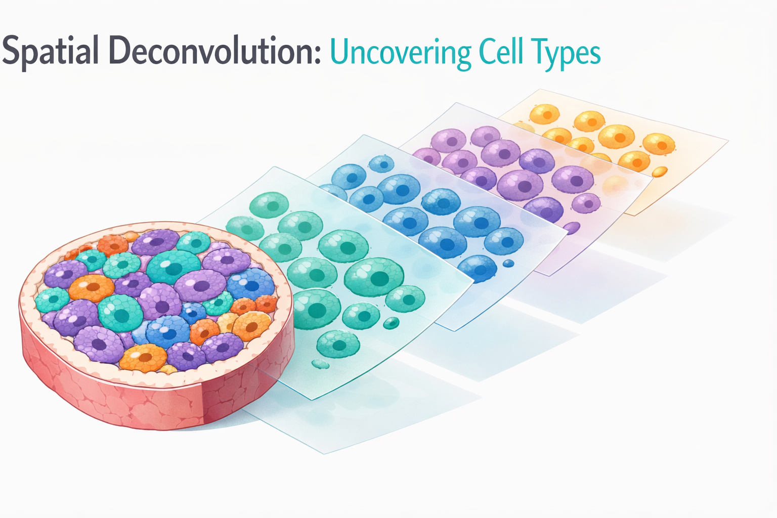
Spatial transcriptomics lets you measure gene expression while preserving where it happens in tissue. But there’s a catch: each region you measure isn’t a single cell type — it’s a mixture.

That means every expression profile is an average across many cells — and averages can be misleading. This is known as the cellular mixing problem in spatial transcriptomics, and it’s one of the most important challenges to address before drawing biological conclusions from platforms like NanoString’s GeoMx Digital Spatial Profiler (Merritt et al., 2020).

That’s where spatial deconvolution comes in.

What Is Spatial Deconvolution?

Spatial deconvolution is a computational method that estimates the proportions of different cell types within a spatially-defined tissue region. Think of it like reverse-engineering a smoothie: you know what the final mixture tastes like, but you want to figure out how much of each fruit went into the blend.

In molecular terms, each ROI in a GeoMx experiment captures a bulk gene expression signal from potentially dozens of cell types — T cells, macrophages, fibroblasts, epithelial cells, and more. Deconvolution algorithms use reference expression profiles of known cell types (such as the safeTME matrix) to estimate how much each cell type contributes to the observed signal.

Why Does It Matter?

Understanding cell type composition is critical for answering biological questions that go beyond simple gene expression:

• Tumor immunology: Is a tumor region infiltrated by cytotoxic CD8+ T cells, or is it dominated by immunosuppressive regulatory T cells? The gene expression profile alone may not tell you, but deconvolution can.
• Disease progression: How does the cellular landscape of a tissue change as disease advances? Tracking shifts in cell type proportions across disease stages can reveal when immune infiltration begins or when fibrosis takes hold.
• Biomarker validation: A gene that appears upregulated in a tissue ROI might actually reflect a change in cell composition rather than a change in per-cell expression. Deconvolution helps disentangle these effects.

Without deconvolution, you risk attributing changes in gene expression to biology when they’re actually driven by shifts in cell composition.

How It Works: The SpatialDecon Approach

The Bioconductor package SpatialDecon (Danaher et al., 2022) is one of the most widely used tools for this task. At its core, SpatialDecon models each ROI’s expression as a weighted combination of known cell type signatures — solving a regression problem to find the mixture proportions that best explain the observed data. The general workflow involves:

1. Loading raw count data from GeoMx exports (TargetCountMatrix, SegmentProperties, TargetProperties)
2. Background correction using negative control probes to estimate technical noise
3. Normalization — typically Q3 (upper quartile) normalization to account for differences in sequencing depth across ROIs
4. Deconvolution using a reference profile matrix that contains expected expression signatures for each cell type
5. Visualization — heatmaps, PCA plots, and boxplots to interpret the results

The Most Important Decision: Choosing the Reference Matrix

The reference matrix is arguably the most important decision in the entire workflow. NanoString provides the safeTME (safe Tumor Microenvironment) matrix, which includes signatures for 17+ immune and stromal cell types (Danaher et al., 2022). For non-human studies, researchers often turn to species-specific cell atlases.

A poorly matched reference — for example, using a pan-tissue reference when studying kidney — can lead to inaccurate or misleading estimates. Whenever possible, use a tissue-specific or disease-specific reference that reflects the biology you expect to find.

Background Correction: To Correct or Not?

One underappreciated decision is how to handle background signal. GeoMx experiments include negative control probes that estimate non-specific binding. You can use these to perform background correction (the geomx_bg mode in SpatialDecon), or you can skip background correction and use CPM normalization instead.

In our experience, the right choice depends on the signal-to-noise ratio of your dataset. When the background-to-signal ratio is high (approaching 1.0), background correction can remove too much real signal. In these cases, CPM normalization without background correction often produces more biologically interpretable results.

The key insight: when background approaches signal, correction can do more harm than good.

Practical Tips from Our Work

Having applied spatial deconvolution across multiple GeoMx projects — spanning cancer immunology, kidney disease, and immune profiling — we’ve developed several practical guidelines:

1. Never trust deconvolution results without validating against known biology. If you profiled ROIs using a marker like CD3 (T cells) or PanCK (epithelial cells), check whether the deconvolution estimates align with what you’d expect from that marker.

2. Compare multiple normalization approaches. Run deconvolution with both background-corrected and CPM-normalized data, then compare. If the results are concordant, you can be more confident in the findings. If they diverge, investigate why.

3. Consider compartment-specific analysis. In studies where you’ve profiled multiple tissue compartments (e.g., tumor, stroma, immune), analyze each compartment separately rather than pooling everything together. Cell type proportions in a tumor region have very different biological meaning than cell type proportions in adjacent stroma.

4. Watch for low-abundance cell types. Deconvolution estimates for rare cell types (e.g., mast cells, dendritic cells) are inherently noisier. Be cautious about drawing strong conclusions from small estimated proportions.

Limitations to Keep in Mind

Deconvolution is powerful, but not perfect. It depends heavily on the quality of the reference matrix — garbage in, garbage out. It cannot identify unknown cell types that aren’t represented in your reference. And it’s sensitive to preprocessing choices like normalization and background correction. Always treat deconvolution estimates as informed approximations, not ground truth.

Looking Ahead

As spatial biology platforms continue to mature — with higher resolution, more multiplexing, and deeper coverage — deconvolution methods will become even more important. Emerging approaches that integrate single-cell RNA-seq reference data with spatial profiles are already pushing the boundaries of what’s possible.

These considerations aren’t theoretical — they show up in nearly every spatial dataset we analyze. At Cytogence, spatial deconvolution is a core part of our GeoMx analysis pipeline. Whether you’re studying tumor-immune interactions, disease progression, or tissue remodeling, understanding the cellular composition of your spatial data is the foundation for meaningful biological insight.

References

1. Danaher P, Kim Y, Nelson B, et al. Advances in mixed cell deconvolution enable quantification of cell types in spatial transcriptomic data. Nature Communications. 2022;13:385. doi: 10.1038/s41467-022-28020-5. PMID: 35046414.

2. Merritt CR, Ong GT, Church SE, et al. Multiplex digital spatial profiling of proteins and RNA in fixed tissue. Nature Biotechnology. 2020;38(5):586-599. doi: 10.1038/s41587-020-0472-9. PMID: 32393914.

---

Cytogence specializes in bioinformatics consulting for spatial transcriptomics, multi-omics integration, and high-throughput biology. Contact us to learn how we can support your research.