Power Analysis for Omics Studies: Sizing Experiments Before You Spend the Grant

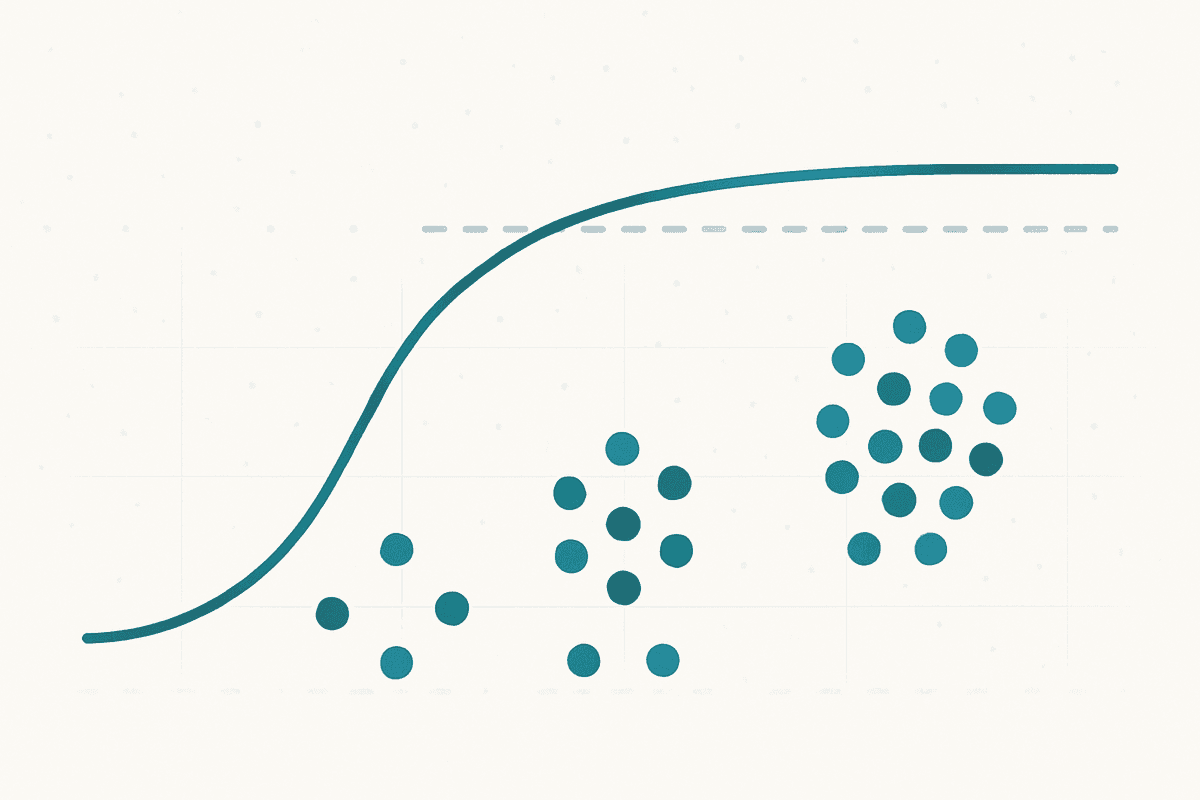
The most expensive mistake in an omics project is usually made before a single sample is sequenced. A lab inherits “n=3 per group” as a default — it’s what the last paper did, and it fits the budget once you account for animal or tissue availability, per-sample sequencing cost, and a grant that’s stretched thinner every year — runs the experiment, and only at the analysis stage discovers there isn’t enough signal to call anything significant after multiple-testing correction. The data are real. The biology may even be there. But the study was never sized to see it — and by then the grant money is spent. This isn’t carelessness; small n is usually a rational response to real-world constraints. The problem is that those constraints get applied without checking whether the resulting study can actually answer the question.

We get pulled into a fair number of these conversations after the fact, asked to “rescue” an analysis that no method can rescue. The honest answer is that power is a design-time decision, not an analysis-time one. Here’s how we think about sizing transcriptomics and other omics experiments, why the calculator you used for a t-test will mislead you, and the trade-offs that actually move the needle.

Why textbook power calculations break for omics

The power analysis most people learned assumes one outcome, a known effect size, and a known variance. You plug in α, the difference you want to detect, and the standard deviation, and out comes a sample size. Clean.

An RNA-seq experiment violates every one of those assumptions:

• You’re not testing one hypothesis — you’re testing tens of thousands. Twenty thousand genes means twenty thousand tests, and controlling the false discovery rate (FDR) at 5% imposes a far steeper significance bar than a single α = 0.05. Power has to be defined as “the proportion of truly differential genes you expect to detect at your chosen FDR,” not the power of one test.
• There is no single effect size. Genes span a huge range of fold changes, and the ones you care about are often the modest ones.
• Variance isn’t a constant — it’s a function of expression. Count data are well described by a negative binomial distribution, and the dispersion (the biological-plus-technical variability around the mean) changes with expression level. The mean–dispersion relationship is the thing that governs power, and it’s different in every tissue and platform.

Crucially, for the low-fold-change genes that are usually the interesting ones, biological variability and sample size dominate power far more than read depth does (Wu et al., PROPER). This is really a budget-allocation decision, and it’s worth settling early: a sequencing run buys you a fixed pool of dollars to split between how many samples and how deep per sample. Past a modest depth, adding reads buys you very little; once each library is sequenced deeply enough, the next dollar is almost always better spent on another biological replicate than on deeper sequencing of the samples you already have. The single most common design error we see is the opposite call — money poured into deeper sequencing of too few samples.

Pilot data beats a guessed effect size

Because dispersion is dataset-specific, the most defensible power estimates come from simulation grounded in pilot data rather than a number you typed into a parametric formula. The workflow is: take a small pilot (or a public dataset from comparable tissue and platform), estimate the real mean–dispersion relationship, then simulate experiments at a range of sample sizes and measure how often you recover the genes you planted.

Several mature, freely available tools do exactly this for bulk RNA-seq:

• PROPER (PROspective Power Evaluation for RNAseq) runs simulation studies across a range of sample sizes and reports both power and the actual realized type-I error.
• RNASeqPower gives a faster analytic estimate when you can supply a coefficient of variation and target effect size.
• powsimR simulates from a negative-binomial model that explicitly captures the mean–dispersion relationship, and handles both bulk and single-cell designs.

None of these is a black box you trust blindly, and none of this is a checkbox. Estimating a defensible mean–dispersion relationship from pilot or comparable public data, parameterizing a realistic simulation, and reading the resulting power curves with judgment is genuine analyst work — a meaningful task done well, not a number you read off a calculator in five minutes. That’s the honest trade-off, and it’s the whole argument for doing it: good design costs real effort up front, but it’s far cheaper than discovering after the money is spent that the study was never powered to answer the question. The point of running these tools on your pilot is that the dispersion estimate reflects your tissue, your library prep, and your batch structure — not an idealized organism. If you have no pilot and no comparable public data, that’s worth knowing too: it means your sample size is a guess, and you should budget conservatively and say so.

For a fuller treatment of the underlying statistics across bulk, single-cell, and spatial designs, the 2023 Biomolecules review by Jeon et al. is a good current reference.

Single-cell changes the question entirely

Single-cell and single-nucleus experiments add a dimension that bulk power analysis doesn’t have: you’re now choosing how many cells per sample and how deeply to sequence each cell, on top of how many biological samples (donors) to run. These trade off against each other under a fixed budget, and the intuition from bulk doesn’t carry over.

The clearest result here comes from scPower (Schmid et al., Nature Communications, 2021), a framework built specifically for multi-sample single-cell design. Its headline finding is counterintuitive and budget-relevant: for detecting cell-type-specific differential expression and eQTLs, shallow sequencing of many cells generally yields higher power than deep sequencing of few cells (Schmid et al., 2021). It also makes the often-overlooked point that for a rare cell type, your effective sample size is the number of cells of that type per donor — you can be richly powered for a common population and badly underpowered for the one you actually came to study.

Note the design distinction that trips people up: in a population-scale single-cell study, the unit of biological replication is the donor, not the cell. Thousands of cells from three donors is, for many inter-individual questions, an n of 3 — a point we’ve made before in when to reach for single-cell versus bulk or spatial. Tools like POWSC and scPower help you reason about this explicitly rather than being lulled by a large cell count.

Spatial transcriptomics is earlier in its tooling, but the same simulation-from-pilot philosophy is being extended to it — methods such as PoweREST, now published in PLOS Computational Biology (2025), estimate power for spot-level differential expression. Even with peer-reviewed tooling arriving, we’d still treat spatial power estimates as more provisional than bulk ones today and design with margin.

The decisions that actually move power

Stepping back from tools, a handful of design choices dominate whether your study succeeds:

• Biological replicates over technical depth. For almost every differential-expression question, the next replicate is worth more than the next 10 million reads. Spend there.
• Control the variance you can control. Power is inversely tied to dispersion, so anything that reduces unwanted variability — consistent sample handling, matched processing batches, tighter inclusion criteria — directly buys power. And don’t confound: if every treated sample is processed on a different day than every control, no sample size and no batch-correction method can fully separate the effects.
• Define the effect that matters. “Detect any difference” isn’t a design target. Powering to detect a two-fold change in well-expressed genes is a very different (and cheaper) experiment than powering for 1.3-fold changes in a rare cell type. Decide which one you actually need.
• Power for the analysis you’ll run. If the real question is an interaction, a cell-type-specific contrast, or a subgroup, power for that, not for the marginal comparison — the subgroup is always the underpowered one.

None of this requires exotic statistics. It requires deciding the question precisely, getting a realistic variance estimate, and being honest when the budget can’t support the question — sometimes the right call is a smaller, well-powered study over a sprawling, underpowered one.

Get it right before the data exist

Power analysis is unglamorous and easy to skip under grant-deadline pressure. But it’s one of the highest-leverage hours in the entire project: it’s the difference between a dataset that answers your question and one that merely exists. It also belongs in the project’s statement of work — sizing assumptions written down at the start protect both the science and the budget.

If you’re designing an omics experiment and want a sanity check on sample size before you commit the grant — bulk, single-cell, or spatial — that’s exactly the kind of pre-data consulting we do. An hour spent here is far cheaper than a re-run later.

References

• Schmid KT, et al. “scPower accelerates and optimizes the design of multi-sample single cell transcriptomic studies.” Nature Communications, 2021. 10.1038/s41467-021-26779-7
• Vieth B, et al. “powsimR: power analysis for bulk and single cell RNA-seq experiments.” Bioinformatics, 2017. github.com/bvieth/powsimR
• Wu H, et al. PROPER: PROspective Power Evaluation for RNAseq. Bioconductor
• Jeon H, Xie J, Jeon Y, et al. “Statistical Power Analysis for Designing Bulk, Single-Cell, and Spatial Transcriptomics Experiments: Review, Tutorial, and Perspectives.” Biomolecules, 2023;13(2):221. PMC9952882